I Built a Forecasting Engine for Shillong Teer. The ML Model Lost to Physics.

Every working day in Shillong, two rounds of archers shoot at a cylindrical target. Count the arrows that land, take the last two digits, and you have the day's Teer result — a number from 00 to 99. People bet on it. A correct pick pays roughly 79 to 1.

Most people treat it like a lottery. But it isn't a random number generator. It's aggregated human-athletic performance — a dozen clubs, real archers, real fatigue, real schedules. And anything generated by humans on a schedule probably carries structure.

So I spent two years collecting data and building TeerML: a walk-forward probabilistic forecasting engine that scores all 100 digits for both rounds, every match day. This is the story of versions 6.0 through 6.4 — including the part where the machine learning model lost to a handful of Gaussian priors.

The signal hypothesis

Why would Teer results be predictable at all? Five reasons kept showing up in the data:

• —Club consistency — each club's archers have characteristic accuracy distributions that drift slowly.
• —Rest effects — how a club performs correlates with how long it's been since their last appearance, and what they shot last time.
• —Fatigue — clubs that appear frequently in a short window produce tighter, more clustered results.
• —Head-to-head dynamics — specific club pairings behave differently than each club's unconditional history.
• —Target physics — the target's cross-section changes between rounds; a bigger target should mean more arrows landing.

The catch: any model exploiting these has to be honest about time. Predictions for date t can only use data from strictly before t. No lookahead, ever. Every version below was evaluated under the same walk-forward backtest, with a 60-day warm-up and the entity index rebuilt fresh at every step.

hist = all_results[date < t]   # the only temporal guard you need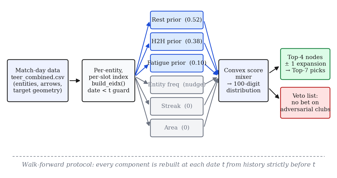

The architecture

The core idea is simple: for each club on each day, build several candidate probability distributions over digits 0–99 from complementary signals, then mix them into one score per digit. Six priors:

• —Entity frequency — time-decay-weighted histogram of the club's past results (half-life 180 days)
• —Head-to-head (H2H) — the same, restricted to this exact club pairing (minimum 5 co-appearances)
• —Rest prior — the interesting one, more below
• —Fatigue prior — a Gaussian around the recent 14-day mean that narrows as appearance density rises
• —Streak — momentum over the last 8 appearances
• —Area prior — shifts the expected result when today's target is bigger or smaller than the club's historical average

The rest prior is the whole game

The rest prior models a tension between two regimes. After a short gap (< 4 days), a club tends to carry over its last result — so the prior is a Gaussian centred on the last result. After a long gap (> 10 days), it reverts to the club's historical mean. In between, blend linearly:

α          = clip((rest_days − 4) / 6, 0, 1)
rest_prior = α · N(entity_mean, σ) + (1 − α) · N(last_result, 0.6σ)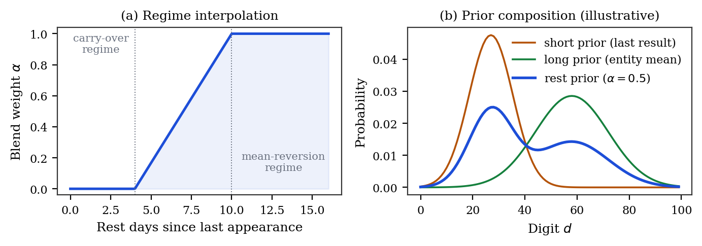

This is fatigue-recovery dynamics at a coarse time scale, the same pattern you see all over human athletic performance data. Hold that thought — it matters in a minute.

Six versions, one plot twist

v6.0 was a hand-weighted mixer: 40% entity frequency, 25% H2H, 20% streak, 15% area. Pick the top 5 digits. A reasonable baseline. v6.1 added the rest and fatigue priors at a timid 5% each. v6.2 is where it got interesting. I ran a two-stage optimisation: a 45-configuration grid search over structural parameters (decay half-life, H2H threshold, streak window), then 2,000 Dirichlet-sampled weight vectors for each of the top five configs, all evaluated through the full walk-forward backtest. The optimiser tore up my hand-set hierarchy:

rest    0.41   ← dominant
h2h     0.31
fatigue 0.21
entity  0.04   ← nearly gone
streak  0.02
area    0.01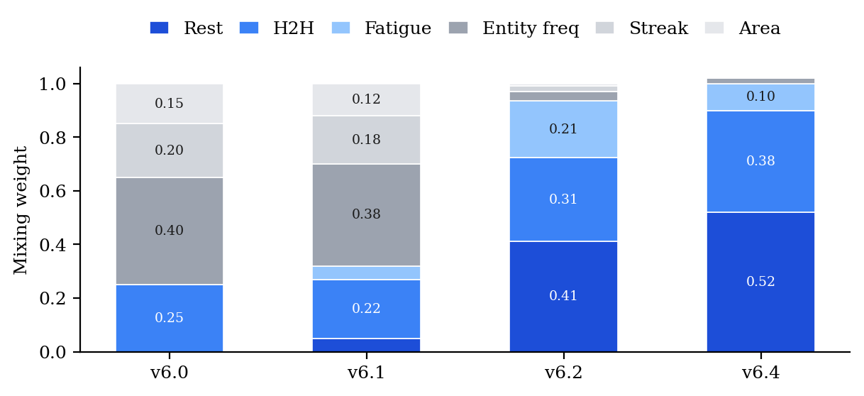

Everything I'd weighted heavily — raw frequency, momentum — was noise. The game's dominant structure is rest-day mean-reversion.

v6.3 was the obvious next move: replace the hand-mixed priors with a LightGBM classifier. 29 features per digit, scoring every (date, digit, entity) triple, softmax over all 100 digits, batch retraining every 20 dates with strict walk-forward hygiene. It performed worse than v6.2. With only ~300–500 training rows, gradient boosting couldn't out-learn the inductive bias already baked into the physics priors. The classifier's feature importances actually agreed with the heuristic's hierarchy — rest, H2H, fatigue on top — it just couldn't exploit them without overfitting entity-level noise.

"needs ~1500+ rows to beat physics model."

The priors don't need to learn fatigue-recovery dynamics from scratch; they assume them. At small data scales, a good assumption beats a flexible learner.

v6.4: weight surgery and knowing when not to bet

The final version is deliberately reductionist. Three primary weights — Rest 0.52, H2H 0.38, Fatigue 0.10 — with entity frequency demoted to a +2% tie-breaking nudge. Streak and area: deleted. Two additions did the heavy lifting:

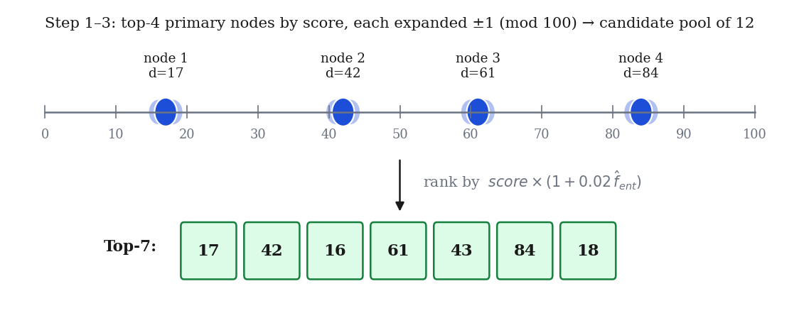
±1 node expansion. Backtests showed a persistent near-miss pattern — a large share of rounds landed within ±2 digits of the model's nearest pick, with mean circular distance far below the ~25 you'd expect from random guessing. So instead of betting the raw top 5, v6.4 takes the top 4 primary nodes, expands each by ±1 (mod 100 — digit 99 is adjacent to digit 0), and bets the best 7 from that pool.

The veto list. Entity-level analysis showed that for certain clubs, the model has no edge — sustained negative Sharpe over 20+ appearances. Rather than pretending otherwise, v6.4 simply refuses to bet when those clubs are scheduled. Four R1 clubs, four R2 clubs, capital preserved. The most profitable feature in the whole system might be the one that does nothing.

Five iterations. Every number moved the right direction.

+3.3 POINTS ABOVE RANDOM. IN A 100-DIGIT GAME, THAT'S A REAL EDGE.

What I'd tell you if you're building something similar

The honest caveats: the dataset is still small (~300–700 usable rows), clubs are non-stationary — archers change, venues change — and the backtest assumes flat unit stakes with no Kelly sizing. All of that is future work.

But the central finding stands: an archery lottery, of all things, has exploitable structure — and it's not hiding in the frequencies everyone stares at. It's in the rest days.